Why My Model Trained Differently on a CPU and a GPU

A couple friends and I took it upon ourselves to start a project that pertained to trading. After reading a paper that used machine learning to forecast weather, we built our own model to predict daily high temperatures in New York City. I trained a Temporal Fusion Transformer (TFT), alternating between an Apple Silicon Mac and a Windows machine with an NVIDIA GPU. Using the same seed, hyperparameters, and training data, I expected both runs to converge to the same solution. Instead, they consistently produced different outputs.

When I first encountered non-reproducible training runs I suspected the seeds, data shuffling, dropout. The more fundamental source of variation is the floating-point arithmetic itself. This boils down to the hardware level and how it is executing the matrix multiplication.

IEEE 754 and the illusion of a continuum

Understanding how modern hardware represents floating-point numbers is the first step. IEEE 754 is the standard for floating-point arithmetic. This standard represents a number using 32 bits. The anatomy is: 1 sign bit, 8 exponent bits, and 23 mantissa bits.

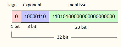
What matters is not just how these bits encode a number, but what this structure implies for computation itself. The exponent determines scale. The mantissa determines precision at that scale. Together, they define a system that does not represent the real number line continuously, but instead discretizes it into uneven steps. Near zero, those steps are extremely small; as magnitude increases, the spacing between representable numbers grows rapidly.

So unlike real arithmetic, where numbers exist on a continuous line, floating-point arithmetic lives on a quantized approximation of that line. Every operation has to “snap back” to the nearest representable value. That snapping is where error enters.

Associativity breaks down

This changes a fundamental assumption in algebra. In real numbers, operations like addition are associative:

$$(a + b) + c = a + (b + c)$$

In floating-point arithmetic, this is no longer guaranteed because every operation has to “snap” to the nearest representable value. Mathematically, you can think of this as projecting the result back onto the floating-point lattice, or rounding:

$$\mathrm{fl}(\mathrm{fl}(a + b) + c) \ne \mathrm{fl}(a + \mathrm{fl}(b + c))$$

The important point is not just that this equality breaks, but why it breaks: every intermediate result is being projected back onto a finite-resolution grid defined by the mantissa. That rounding depends on magnitude, ordering, and how values align within the representable spacing.

In practice, this means that floating-point arithmetic is not just “real arithmetic with small errors.” It is a sequence of deterministic operations interleaved with structured information loss.

Gradient descent as a dynamical system under rounding

From this perspective, gradient descent stops being a clean deterministic update rule and becomes a dynamical system under repeated rounding:

$$\theta_{t+1} = \theta_t - \eta \nabla L(\theta_t)$$

In exact arithmetic, this trajectory is fixed. But in floating-point arithmetic, every evaluation of $\nabla L$ includes many intermediate roundings—matrix multiplications, reductions, nonlinearities—all of which introduce small, structured perturbations. The update rule becomes:

$$\theta_{t+1} = \theta_t - \eta (\nabla L(\theta_t) + \delta_t)$$

where $\delta_t$ is the accumulated effect of finite-precision rounding across the computational graph.

Once you see computation this way, the hardware differences become meaningful. The question is no longer just “do we compute the same function,” but “do we generate the same sequence of roundings onto the representable number line.” And this is exactly where CPU and GPU begin to diverge.

Where rounding starts to matter: aggregation

Where does this rounding actually start to matter in deep learning systems? The answer is not in isolated arithmetic operations. It appears in aggregation.

One of the first places floating-point behavior becomes visible is during reduction operations: summing gradients, accumulating partial results, and merging updates across batches and threads.

At this point we know two things. First, every floating-point operation introduces a tiny rounding error. Second, the result depends on the order in which operations occur. That naturally leads to the next question: who decides the order? The answer is the hardware. CPUs and GPUs perform the same mathematical operations, but they organize those operations very differently. Those differences are where identical training runs begin to diverge.

How does a CPU approach reduction?

On a CPU, reduction is largely sequential or deterministically vectorized. Even when SIMD instructions are used (AVX, AVX2, AVX-512), the structure of the computation is still fundamentally ordered. A fixed instruction sequence defines how partial sums are combined, and that sequence does not change across runs.

So even though each addition still involves rounding, the path through the number line is stable. The same values are combined in the same order, meaning the same intermediate roundings occur in the same places. As a result, the accumulated rounding error is consistent. It may not be “correct” in a mathematical sense, but it is reproducible.

Reproducibility here is not about precision. It is about determinism of error.

How does a GPU approach reduction?

A GPU breaks this structure entirely. Instead of a single ordered reduction, computation is distributed across thousands of threads. Each thread computes a partial result, and those results are combined asynchronously through shared memory.

At the center of this mechanism are atomic additions. An atomic add ensures that multiple threads can safely update a shared value without explicit locking. It does not guarantee ordering.

Two runs of the same kernel can produce different effective summation orders because thread scheduling is not fixed at the hardware level. Warps are executed in parallel across streaming multiprocessors, and their completion order depends on factors like occupancy, memory latency, and instruction pipeline timing.

So instead of a fixed expression like:

$$((a + b) + c) + d$$

the system effectively explores different valid permutations of the same reduction:

$$\begin{gathered} (a + (c + d)) + b \\ ((a + d) + b) + c \\ (b + (a + c)) + d \end{gathered}$$

In exact arithmetic, these expressions are equivalent. In floating-point arithmetic, they are not.

Why does ordering change the result?

Recall mantissa geometry. Each floating-point number carries a fixed amount of precision relative to its magnitude. When two numbers differ significantly in scale, the smaller value may fall outside the representable precision of the larger one and effectively disappear during addition.

So if a large partial sum is accumulated first, smaller contributions added later may be partially or fully lost. But if those small values are accumulated earlier—before being merged into a large magnitude term—they may survive the rounding step and persist into the final result.

This means that summation is not just aggregation. It is a sequence of information retention and information loss events, and that sequence depends entirely on order.

Across a single gradient update, this difference is usually tiny. Often sub-ULP. But in a deep network, this process is repeated millions or billions of times. Each update slightly shifts the trajectory of the parameters, not randomly, but path-dependently. Over time, these small divergences accumulate into different optimization paths entirely.

The core issue

This is the key distinction: in a deterministic CPU implementation, the reduction path is fixed from run to run. GPUs, by contrast, often allow many valid reduction orders to emerge naturally from parallel execution.

And in floating-point arithmetic, “valid” does not mean “equivalent.” It only means “within rounding error at each step.” Once those rounding decisions are chained together across large reductions, the system becomes sensitive to ordering in a way that cannot be eliminated without changing the algorithm itself.