The Persuasion Ceiling

Update, November 2026. The 3 seats this post ends on didn’t hold up either. The ceiling treated a symptom: the first dollar’s effect blew up because returns were measured in share of spending. Rebuilt with returns that shrink with each added dollar, and using only what a committee could know by September, DCCC’s spending comes within 0.05–0.19 expected seats of the best use of its budget. See Campaign Allocation. I’ve also corrected the derivative below, which used Φ where the normal density φ belongs, and a claim about the ceiling’s shape.

In Political Theta I described how this project started: a House-race allocation model built on free FEC campaign finance data, including the DCCC’s own filings, aimed at one target, whoever wins the most House seats.

With that target set, I evaluated several allocation strategies against the same campaign budget: the DCCC’s actual 2024 spending, an equal split across every congressional race, an allocation weighted by Cook Political Report race ratings, and a nonlinear optimizer that maximized expected House seats directly.

The optimizer’s result was nearly 13 extra seats. Considering the polarization between both parties, imagine if a simple reshuffling of the same budget handed one party an overwhelming House majority. That’s suspiciously optimistic. Either I’d found a gaping inefficiency in how the DCCC spends money, or my model had extrapolated gains well beyond what the data could support.

The optimizer itself is simple. It maximizes expected seats:

$$E[\text{Seats}] = \sum_i \Phi\big(\mu_i(D_i) / \sigma_i\big)$$

In English: for every race $i$, take the expected Democratic margin after spending $D_i$ dollars, divide by that race’s uncertainty, and pass it through the normal CDF to get a win probability. Sum those win probabilities across every race and you get expected seats. The optimizer allocates capital wherever the marginal improvement is largest.

To understand why it returned something as optimistic as 13 seats, I took the partial derivative of that equation with respect to spending and applied the chain rule:

$$\frac{\partial}{\partial D} \Phi\big(\mu_i(D_i) / \sigma_i\big) = \phi(\mu/\sigma) \cdot (1/\sigma) \cdot \partial\mu/\partial D$$

That splits one hard question into three easier ones:

1. $\phi(\mu/\sigma)$, the normal density, positions a race on a bell curve based on spending and partisan lean, to determine how competitive it is. A safe race for either party sits out in a tail, where the curve is nearly flat, because its expected margin is far from zero; a toss-up sits near the center, where the curve is tallest. This follows an assumption I made, that safe or likely races are close to deterministic.
2. $1/\sigma$ is the uncertainty weight per race. As long as a race has genuine uncertainty, which I assumed to be true everywhere until a winner is actually seated, this term stays finite and helps stabilize the optimizer.
3. $\partial\mu/\partial D$ is the margin response: how much expected margin moves per dollar spent. As spending approaches zero, this term approaches infinity. At first glance that seems correct, more competitive dollars matter more, but the byproduct is an unbounded optimizer that produces untrustworthy results.

The tension is between the first term, which wants to minimize allocation in races that are already decided, and the third term, which insists the very first dollar spent anywhere is infinitely valuable. That tension is supposed to balance out. It didn’t.

Before I understood any of this, I went digging through my own codebase, convinced I’d accidentally swapped in an older linear optimizer, since fitting a straight line to this kind of data reliably produces overly optimistic results too. That wasn’t it. I recomputed expected seats independently, using only the optimizer’s recommended allocation and the win-probability equation on its own. Same answer. The optimizer was doing exactly what it was told to do.

I went back to look at the data to understand what the optimizer was seeing and how the capital was split between categories in safe, likely, lean, and tossup races. The results were striking. Roughly 81% of the optimizer’s projected seat gain came from races that had historically spent less than $500,000. Even more concerning, roughly 45% of the recommended party budget flowed into Safe-tier races, despite those races being the least likely to determine control of the House.

The delicate balance wasn’t working, because the margin-response term was overpowering the density term. The value of the first dollar was huge everywhere, regardless of the district, and especially huge in races with almost no existing funding. The optimizer had found a source of expected-seat gain that doesn’t exist in reality.

Campaigns have fixed costs. The optimizer assumed spending always has some positive effect no matter how much has already been spent, the gains shrink but never fully vanish. In reality, political services are discrete chunks of spending with limited influence. The optimizer had also implicitly assumed every safe-Republican race sits only slightly underwater. In reality some of those races are 15 points underwater and will not be moved by any amount of money. The model was treating spending as if it always raises win probability, which simply isn’t true once a race is out of reach.

So what to do? I tried a few things. The first was estimating district-level persuadability, using demographics and past swing data to scale down the effect of each dollar by an estimated swing-voter share. That failed for two reasons: the data didn’t exist at the resolution I needed, and even with what I could collect, multiplying a persuadable percentage against infinity just gives you a smaller infinity.

The second idea was to force the optimizer to spend less in safe seats directly, weighting each district by its Cook Political Report race rating: 1.0 for toss-ups, 0.1 for safe seats, something in between for lean and likely. This worked, technically. This changed the problem. I was no longer maximizing total seats won, I was maximizing a number partly defined by Cook’s ratings, which happen to already favor competitive races. This was not the ideal solution.

The fix I landed on came from noticing that the model already has a belief about how likely a district is to go Democratic before a single additional dollar is spent. I didn’t need an external heuristic like PVI, partisan registration, or historical margins. I could define the ceiling endogenously, from the model’s own baseline win probability, $\Phi_0$.

If $\Phi_0 = 0.95$, the model already believes the Democrat wins 95% of the time. How much persuasion does that race need? Almost none. If $\Phi_0 = 0.5$, the race is a true toss-up, and every dollar has potential to tip the balance. Races the model already considers near-certain, in either direction, have very little persuasion left to sell. This is elegant precisely because the ceiling requires no outside data, it’s derived entirely from the model’s internal calculation, and the optimizer becomes self-regulating by design.

For each race, the model computes that baseline win probability as $\Phi_0 = \Phi(\mu_0/\sigma)$, where $\mu_0$ is the predicted margin before any additional spending. Here’s what that looks like for four real 2024 races, comparing the raw, uncapped response to the capped one:

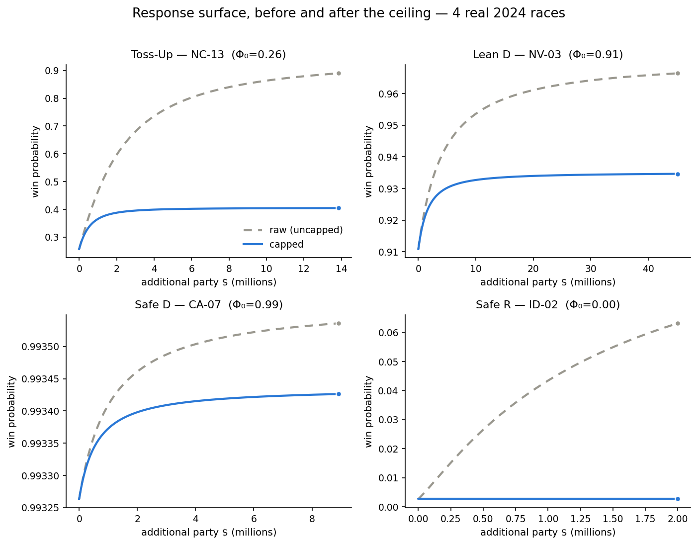
In the toss-up (NC-13), the capped curve still rises meaningfully with more spending. In the two safe races (CA-07 and ID-02), the capped curve flattens almost immediately, exactly the behavior the uncapped model was missing.

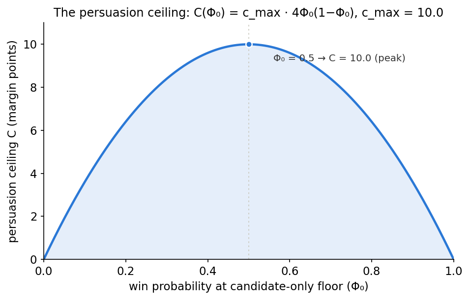
I let the persuasion ceiling depend on the race’s own existing competitiveness:

$$C(\Phi_0) = C_{\max} \cdot 4\Phi_0(1 - \Phi_0)$$

$C_{\max}$ is the most persuasion any amount of money could ever buy, in margin points, and the $4\Phi_0(1 - \Phi_0)$ term peaks at 0.5 win probability and falls to zero at either extreme. So the ceiling itself is highest for toss-ups and collapses toward zero for races that are already decided:

To make sure this wasn’t just a lucky choice of constant, I swept $C_{\max}$ across {3, 5, 7, 10, 15, 20, 30} margin points, meaning anywhere from “money can move 3% of the vote at most” to “money can move 30% of the vote,” which should never actually happen, and reran the full optimization for each value. Across every setting, the optimizer kept prioritizing competitive races, and Safe-tier spending stayed a small share of the total budget, somewhere between roughly 7% and 13% depending on how loose the ceiling was:

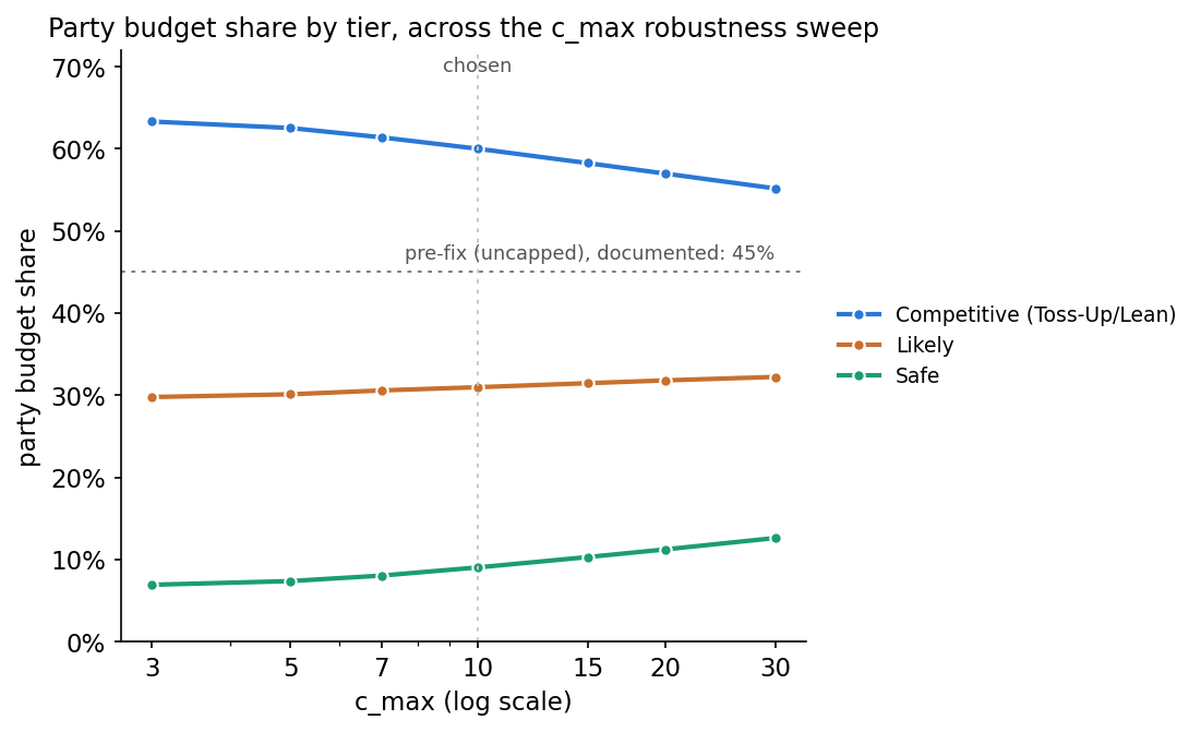
The exact split shifted as the ceiling loosened or tightened, but the optimistic behavior never came back. The ceiling’s shape does favor toss-ups, since it peaks at a 50% baseline by construction. What the sweep shows is that the resulting hierarchy doesn’t depend on how high the ceiling is set, and it matches the intuition of an actual political consultant: safe districts get token amounts, competitive races get the bulk of the money:

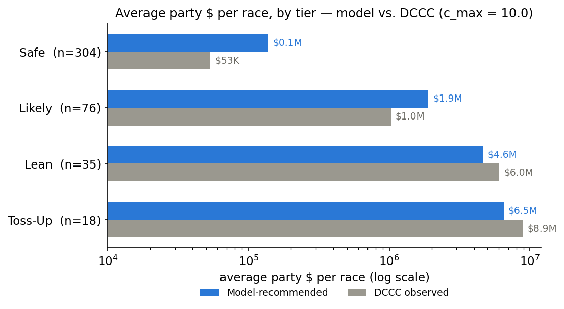
Rerunning the full optimization with the ceiling in place, the 13-seat gain dropped to roughly 3. Far less dramatic, and far more believable.