Asked for 500, Got 40

At work I built a search tool for a political consulting firm’s archive of past campaign pieces: mailers, digital ads, handouts, about 9,800 of them. Claude reads each piece, OpenAI’s text-embedding-3-small turns a labeled summary of it into 1,536 numbers, and Postgres stores those numbers with pgvector. A designer can type something like “seniors worried about Medicare” and get pieces about that idea even when none of them use those words. Under the hood, every search merges two lists: the documents whose vectors sit nearest the query’s, and the documents whose text contains its words. Part 1 covers the embeddings, and part 2 covers pgvector and its HNSW index.

The vector half of that search asked for 500 candidates. I found out it was getting 40 while checking the claims on my portfolio page against the code. There was no error, no warning, and nothing in the logs. When I ran the query against production, the index scan handed back exactly 40 rows.

Forty is not a number that appeared anywhere in my code. It is pgvector’s default for a setting called hnsw.ef_search, a name that also appeared nowhere in my code. The fix turned out to be harder than the bug: raising that setting to 500 made searches take 12 to 21 seconds. Both come down to how an approximate index answers a nearest-neighbor query, and how Postgres decides whether to use that index at all.

ef_search is the size of the answer

Part 2 described how an HNSW search ends. Along the bottom layer of the graph, a best-first search keeps a list of the best candidates it has found, with a fixed capacity, and whatever is on that list when the search stops is the result. In pgvector, that capacity is hnsw.ef_search.

This is the part I had missed. In pgvector 0.7, which production runs, an HNSW index scan returns the contents of that list and then stops. It cannot return more than $ef$ rows, whatever the query asks for:

$$\text{rows returned} = \min(\text{LIMIT},\ ef_{\text{search}})$$

Here is the vector half of the search as it was:

# LIMIT forces HNSW index usage (ORDER BY distance LIMIT N),
# turning O(N) sequential scan into O(log N). Without this,
# pgvector ignores the HNSW index entirely.
_vector_candidates = max(500, per_page * 20)
vector_subquery = (
    select(
        Document.id.label("id"),
        (
            1 - Document.search_vector.cosine_distance(query_embedding)
        ).label("vector_relevance"),
    )
    .filter(Document.search_vector.isnot(None))
    .order_by(Document.search_vector.cosine_distance(query_embedding))
    .limit(_vector_candidates)
    .subquery()
)

With 20 results per batch, max(500, 20 * 20) is 500. The comment was right about the shape: ORDER BY distance LIMIT N is the one shape pgvector will answer from the index. What it didn’t say, because I didn’t know it, is that the index has its own say in how large N can be. Written as SQL, with the setting that was silently in force made explicit:

-- Never set anywhere, so pgvector's default applied:
-- SET hnsw.ef_search = 40;

SELECT id, 1 - (search_vector <=> :q) AS vector_relevance
FROM documents
WHERE search_vector IS NOT NULL
ORDER BY search_vector <=> :q
LIMIT 500;  -- the bound I wrote; the index applies a second one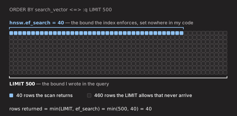

LIMIT is an upper bound the database honors. ef_search is a second upper bound the index enforces without telling anyone, and the smaller of the two wins.

Filters run after the walk

On its own, the cap would have been a modest recall problem. Filters made it a serious one. The search page filters by client, state, year, and topic, and in the old query those filters ran after both lookups came back. HNSW knows nothing about filters. It walks the graph by distance alone, returns its 40, and only then does Postgres discard the rows that don’t match. Here is that flow for a search filtered to one state, as it was built:

flowchart TD
  start([Start]) --> search["Staff member searches “school funding”<br/>and picks one state"]
  search --> embed["Search service embeds the query"]
  embed --> walk["<b>Vector lookup</b><br/>HNSW walks the whole catalog<br/>and returns the 40 nearest pieces"]
  walk --> keyword["<b>Keyword lookup</b><br/>every piece containing “school” and “funding”"]
  keyword --> merge["Merge the two lists and score each piece"]
  merge --> filter["<b>Filter</b><br/>keep only pieces from the chosen state"]
  filter --> show["Show the first 20"]
  show --> scroll{"Staff member<br/>scrolls?"}
  scroll -- Y --> left{"Pieces left in<br/>the filtered list?"}
  left -- Y --> next["Show the next 20<br/>from the same list"]
  next --> scroll
  left -- N --> done([End])
  scroll -- N --> done
  classDef cap stroke:#8fc1f0,stroke-width:2px
  class walk,filter cap

The two highlighted steps are the problem. The vector lookup is capped before the filter ever runs, so the filter can only shrink an already small list. If a filter keeps a fraction $s$ of the catalog, and has nothing to do with the query’s meaning, the expected number of semantic matches that survive is:

$$E[\text{matches}] = ef_{\text{search}} \times s$$

A filter that keeps 10% of the catalog leaves about 4 of the 40. A single client’s pieces are a far smaller slice than that, so a client filter could easily leave the semantic half of the search with nothing at all. The keyword side had no such cap, so a filtered search could come back as nearly all keyword matches.

The scroll loop hit the same ceiling. Every batch drew from the same 40 nearest documents, so a search whose words appeared in no document, one that leaned entirely on meaning, ran out after two batches.

The scoring had a quieter casualty. Each result scored $0.7 \times \text{similarity} + 0.3 \times \text{keyword rank}$, and a keyword match that wasn’t among the 40 nearest got a similarity of zero. A piece containing the exact phrase you typed, sitting 41st by distance, was scored as though its meaning had nothing to do with your query.

None of this produced an error. Vector search always returns something, because there is always a nearest document, so a search never comes back empty and looks broken. The results that did come back really were the 40 closest, so they looked relevant. The failure was in what was missing, and missing results don’t show up in a log.

The obvious fix: ask for 500

If ef_search caps the result, raise it to match the LIMIT. pgvector lets you set it for a single transaction:

SET LOCAL hnsw.ef_search = 500;

I made that change and measured it on production. Semantic searches took 12 to 21 seconds, against about 1.1 seconds for the index scan at the default of 40.

The query plan explained it: there was no index scan anymore. Postgres was reading every vector in the table and sorting them.

Postgres’s planner is cost-based. For each query it estimates what every plausible plan will cost and runs the cheapest. pgvector supplies the estimate for an HNSW scan, and since nothing else about the query had changed, that estimate had to depend on ef_search: a wider search visits more of the graph, so it should cost more. At 500 candidates out of 9,828 documents, the planner priced the walk above reading the whole table. That estimate was wrong. Forced to use the index at a depth of 500, the lookup took 2.5 to 4.4 seconds. But the planner doesn’t know what a plan actually takes. It only knows its own arithmetic.

That full scan was the same one I had escaped in April, when I first gave the query the ORDER BY … LIMIT shape. The obvious fix had quietly put it back.

Forcing the index, and the JIT trap

Postgres has no query hints, but it does have planner switches. Ruling out sequential scans and sorts leaves the HNSW index as the only way to answer ORDER BY distance LIMIT n:

SET LOCAL hnsw.ef_search = 200;
SET LOCAL enable_seqscan = off;
SET LOCAL enable_sort = off;

My first version applied those switches to the whole search. One search took 18.6 seconds, about 12 of them spent compiling the query.

The switches don’t forbid anything. Postgres implements enable_sort = off as a penalty: a plan that sorts anyway has ten billion added to its estimated cost. The vector lookup didn’t need a sort once the index was available, but the rest of the search did. The final step ranks results by a relevance score computed for each query, and no index can hold a number that doesn’t exist until the query runs. So the plan sorted anyway, and its estimated cost became astronomical.

Postgres compiles a query to machine code with LLVM once its estimated cost passes jit_above_cost, and it spends more effort optimizing and inlining as the cost passes higher thresholds. Ten billion passes all of them. On a search for a rare word, compiling added 3 seconds. On a common word, about 12.

The fix was to scope the switches to the one statement that needs them, which meant splitting the vector lookup out of the main query. A planner switch applies to every node in the plan, not just the one you had in mind.

The new search: window, vector lookup, keyword lookup

The search that shipped has three parts, and each answers one question. The window decides how deep to look. The vector lookup finds the nearest pieces at that depth. The keyword lookup finds every piece that matches the words. A final step merges the two, scores them, and returns one batch. Filters no longer run at the end; they go inside both lookups.

flowchart TD
  start([Start]) --> batch["Search page asks for batch p"]
  batch --> window["<b>Window</b><br/>w = min(max(40, 20·(p+1)), 200)<br/>stays at 40 when sorted by date or name"]
  window --> filtered{"Filters<br/>chosen?"}
  filtered -- N --> hnsw["<b>Vector lookup, HNSW</b><br/>ef_search = w; sequential scans and sorts<br/>ruled out for this one statement"]
  filtered -- Y --> exact["<b>Vector lookup, exact</b><br/>the w nearest pieces inside the filters,<br/>ordered by distance + 0"]
  hnsw --> ids["Nearest ids"]
  exact --> ids
  ids --> keyword
  subgraph main ["Main query, one statement"]
    keyword["<b>Keyword lookup</b><br/>every piece matching the words,<br/>inside the filters"] --> merge["<b>Merge</b><br/>candidates = nearest ids ∪ keyword matches"]
    merge --> score["<b>Score</b><br/>0.7 × similarity + 0.3 × keyword rank;<br/>similarity read for the nearest ids<br/>and the w strongest keyword matches"]
    score --> page["Order by score, then id;<br/>return results 20(p−1)+1 to 20p"]
  end
  page --> done([End])
  classDef part stroke:#8fc1f0,stroke-width:2px
  class window,hnsw,exact,keyword part

The window

With the index forced, depth became something I could measure instead of guess. The HNSW lookup alone, on production:

Candidates (ef_search)	Lookup time
40	0.2–1.1 s
100	0.7–1.1 s
200	0.7–1.0 s
500	2.5–4.4 s
Full table scan (the planner’s choice at 500)	12–21 s

Up to 200, the lookup stays around a second. At 500 it is several times slower.

Most searches never get past the first screen, so paying for 200 candidates up front would charge every search for depth that only a scrolling user needs. Instead, the window starts where it always did, at 40, and grows by a batch as the user scrolls:

$$w(p) = \min\big(\max(40,\ 20\,(p+1)),\ 200\big)$$

where $p$ is the batch number, starting at 1, and 20 is the batch size. The first batch draws on 40 candidates, the second on 60, and the ninth reaches the ceiling of 200. Until then, the window always reaches one batch deeper than what has been shown so far.

MIN_CANDIDATES = 40
MAX_CANDIDATES = 200

def _candidate_window(self, page: int, per_page: int, sort_by: str) -> int:
    # A most-relevant list can grow as it scrolls, because what joins it ranks
    # below what is already shown. Sorted by date or name, what joins could
    # land anywhere, so those lists keep the window they start with.
    depth = page if sort_by == "relevance" else 0
    return min(max(MIN_CANDIDATES, (depth + 1) * per_page), MAX_CANDIDATES)

Growing only works when results are sorted by relevance. New candidates come from farther out in the graph, so they mostly rank below what is already on screen and extend the list at the bottom. Sorted by date or name, a new candidate could belong anywhere, including above where the user has already scrolled.

The vector lookup

The vector lookup runs as its own statement and returns a list of ids. It takes one of two paths, depending on whether the search has filters:

def _vector_candidates(self, distance, document_filters, window):
    return (
        select(Document.id.label("id"))
        .filter(Document.search_vector.isnot(None), *document_filters)
        .order_by(distance + 0 if document_filters else distance)
        .limit(window)
    )

def _nearest_document_ids(self, distance, document_filters, window):
    statement = self._vector_candidates(distance, document_filters, window)
    if document_filters:
        return list(self.db.scalars(statement))

    # true: this transaction only, so nothing stays on the pooled connection.
    self.db.execute(select(
        func.set_config("hnsw.ef_search", str(window), True),
        func.set_config("enable_seqscan", "off", True),
        func.set_config("enable_sort", "off", True),
    ))
    nearest_ids = list(self.db.scalars(statement))
    self.db.execute(select(
        func.set_config("enable_seqscan", "on", True),
        func.set_config("enable_sort", "on", True),
    ))
    return nearest_ids

An unfiltered search has to answer from the HNSW index, so it sets ef_search to the window, rules out sequential scans and sorts, runs the lookup, and allows them again before the main query. The settings are transaction-local, so nothing stays behind on the pooled connection.

A filtered search does the opposite and keeps away from the index. Filters are where approximate search hurts most, and also where it is least necessary. A filter shrinks the problem: instead of ranking all 9,828 vectors, the database only has to rank the pieces from one state or one year, which is small enough to do exactly. Ordering by distance + 0 instead of distance is the trick. The two expressions are mathematically identical, but the second is no longer a bare distance operator, so the planner can’t answer it from HNSW. It narrows by the filters first, then computes the exact distance for every row that’s left and sorts. On production, ranking exactly inside the largest state took 0.3 seconds, and inside a single year 1.3 seconds. A filtered search now gets the true nearest pieces within its filter, not whatever survived out of 40.

The keyword lookup

The keyword lookup is a common table expression inside the main query. It applies the same filters as the vector lookup, so both lists are filtered at the source instead of after the merge:

ts_query = func.plainto_tsquery("english", query)
keyword_matches = (
    select(
        Document.id.label("id"),
        func.ts_rank_cd(Document.ts_vector, ts_query, 32)
            .label("text_relevance"),
    )
    .filter(Document.ts_vector.bool_op("@@")(ts_query), *document_filters)
    .cte("keyword_matches")
)

There is no window on this side. The GIN index finds every match exactly, so the keyword lookup returns all of them, however deep the user scrolls. That is also why a common word is still slow, which I come back to at the end.

Merging and scoring

The candidates are the union of the two lists. Every candidate gets a keyword rank, which is zero if it didn’t match the words. Similarity is the expensive part, because it means reading a 6 KB vector, so it is computed only for the nearest ids and for the strongest keyword matches, as many as the window allows. A keyword match outside the nearest set used to count as having no similarity at all and sink below every semantic match. Now the strongest of them are scored on their real meaning:

candidates = union(
    select(Document.id.label("id")).filter(Document.id.in_(nearest_ids)),
    select(keyword_matches.c.id),
)
best_keywords = (
    select(keyword_matches.c.id)
    .order_by(
        desc(keyword_matches.c.text_relevance),
        desc(keyword_matches.c.id),
    )
    .limit(window)
    .subquery()
)
similarity = case(
    (
        or_(
            Document.id.in_(nearest_ids),
            Document.id.in_(select(best_keywords.c.id)),
        ),
        func.coalesce(1 - distance, 0),
    ),
    else_=0,
)
text_score = func.coalesce(keyword_matches.c.text_relevance, 0)
relevance = similarity * 0.7 + text_score * 0.3

The main query then orders by that relevance, with the document’s id as a tie-break, and returns one batch: OFFSET (p − 1) × 20 LIMIT 20. Before the tie-break, documents with equal scores came back in arbitrary order, so a piece could appear twice across batches or never appear at all. The search page also skips any piece it has already shown, which catches the repeat when a newly admitted candidate outranks one already on screen and pushes the list down.

The same ceiling, in CI

The new tests failed on their first run against real pgvector in CI. One expected 80 documents and saw 35. Another found none of its five nearest neighbors.

Each test inserted its documents inside a transaction and rolled it back at the end. A rollback removes the rows but not their entries in the HNSW index. Those stay behind as dead entries until vacuum clears them, and a scan counts them toward ef_search before throwing them away. Earlier tests’ rows sat closer to the shared test query, so they took the slots on the list and were then discarded.

It was the same bug from a different direction. The list is the answer, and anything that takes a slot on it, whether a row a filter will reject or a row that has been deleted, is a result you don’t get. Each test now rebuilds the index inside its own transaction, which the rollback undoes. On production, every depth returned its full count when I measured it.

The core issue

The bug lived in the gap between two layers that each kept their promises. SQL promises that LIMIT 500 returns at most 500 rows. pgvector’s HNSW scan promises the best ef_search candidates its walk can find. Neither promises that a query asking for 500 gets 500, and nothing complains when it doesn’t.

An approximate index changes what a query means. Under an exact plan, ORDER BY distance LIMIT 500 is a specification. Under HNSW, it is a request, answered by a search whose breadth is set somewhere else and whose results filters can only shrink. The obvious fix, widening that search, ran straight into a second layer: a cost-based planner that is free to decide the index isn’t worth using, and to be wrong about it.

Two things are still open. Ranking every match for a common word is the slow path, before and after this change: “vote” matches 7,354 pieces, and scoring all of them takes over 4 seconds. And pgvector 0.8 adds iterative index scans, which keep walking the graph until enough rows survive the filters. That addresses the cap where it starts, inside the index. Production is still on 0.7.2.

LIMIT tells the database how much you want. On an approximate index, it doesn’t tell you how much you’ll get.